North Sea example

This example gives an overview of how to set up a tidal model of the North Sea.

In this demo, we are working with geographic data and so need to import a number of additional packages and configure for the right timezones and map projection. It is common to use UTC as the time zone, since it is used by most observation data sets and domains often cover multiple time zones. For the map projection, we use the UTM coordinate system, which subdivides the surface of the Earth into zones and applies a tangent plane approximation within each zone. In our case, UTM zone 30 is the appropriate one.

from thetis import *
import thetis.coordsys as coordsys
import thetis.forcing as forcing
import csv
import os

sim_tz = timezone.pytz.utc
coord_system = coordsys.UTMCoordinateSystem(utm_zone=30)

Having imported all the relevant packages, the first thing we need is a mesh of the domain of interest. This part is skipped for the purposes of this demo, but details can be found in the corresponding example in the Thetis source code. It involves extracting coastline data from the GSHHS coastline data set [WS96] and using this to generate a mesh using qmesh [ACH+18]. The mesh is stored as a GMSH file named north_sea.msh and is plotted below.

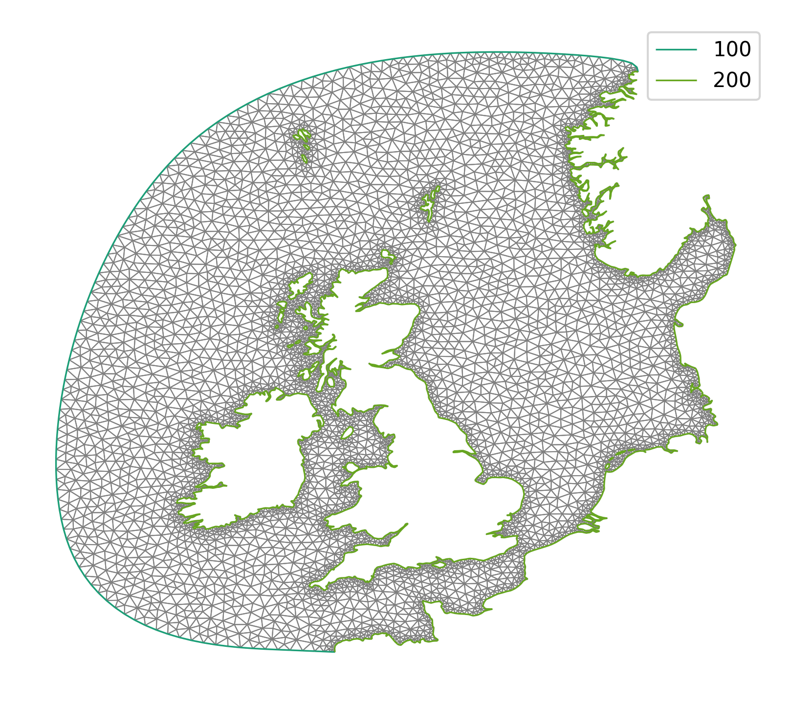
Note that the boundary segments are given different tags, depending on whether they correspond to open ocean (tag 100) or coasts (tag 200). This is because we impose different boundary conditions in each case.

Normally, we would read in this mesh using mesh2d = Mesh('north_sea.msh); Here however, we use a pre-prepared bathymetry that is stored in a checkpoint file and therefore also read in the mesh from the checkpoint file.

For the bathymetry data, we used the ETOPO1 data set [AE09a], [AE09b]. A NetCDF file containing such data for the North Sea can be downloaded from the webpage, stored as etopo1.nc and then interpolated onto the unstructured mesh using SciPy. An interpolate_bathymetry function is provided in model_config module in the example in the Thetis source code, which follows the recommendations in the Firedrake documentation for interpolating data. However, the NetCDF file cannot be included here for copyright reasons, so we insteady provide a HDF5 file containing the data already interpolated onto the mesh. Note that HDF5 files currently have to be saved and loaded using the same number of processors. The bathymetry field was generated by a serial run, so the following will not work in parallel.

with CheckpointFile("north_sea_bathymetry.h5", "r") as f:
    mesh2d = f.load_mesh("firedrake_default")
    bathymetry_2d = f.load_function(mesh2d, "Bathymetry")

The resulting bathymetry field is plotted below.

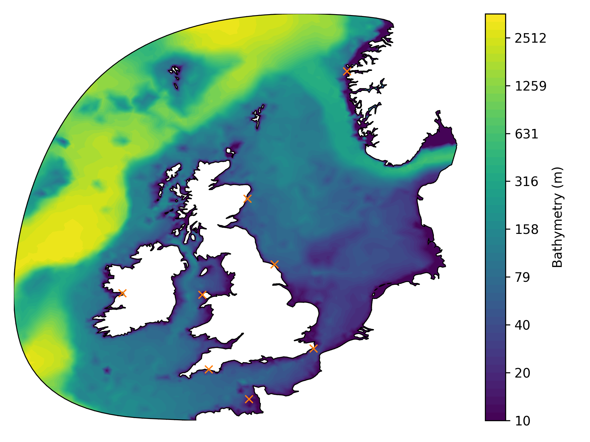
Observe that the plot also includes eight orange crosses. These indicate tide gauges where we would like to compare our tidal model against real data. For details on obtaining such data, we refer to the example in the source code. For the purposes of this demo, we have included a CSV file named stations_elev.csv containing the gauge locations. We can read it as follows:

def read_station_data():
    with open("stations_elev.csv", "r") as csvfile:
        stations = {
            d["name"]: (float(d["latitude"]), float(d["longitude"]))
            for d in csv.DictReader(csvfile, delimiter=",", skipinitialspace=True)
        }
    return stations

We also require fields for the Manning friction coefficient and the Coriolis forcing. These can be set up as follows:

P1_2d = get_functionspace(mesh2d, "CG", 1)
manning_2d = Function(P1_2d, name="Manning coefficient")
manning_2d.assign(3.0e-02)

omega = 7.292e-05
coriolis_2d = Function(P1_2d, name="Coriolis forcing")
lon, lat = coord_system.get_mesh_lonlat_function(mesh2d)
coriolis_2d.interpolate(2 * omega * sin(lat * pi / 180.0))

We also need to choose a time window of interest and discretise it appropriately. We arbitrarily choose the simulation to start at 00:00 UTC on 15th January 2022 and end exactly three days later. We are using a fairly coarse mesh (and will use an implicit time integration scheme) and so can get away with using timesteps of one hour.

start_date = datetime.datetime(2022, 1, 15, tzinfo=sim_tz)
end_date = datetime.datetime(2022, 1, 18, tzinfo=sim_tz)
dt = 3600.0
t_export = 3600.0

We are now in a position where we can create the Thetis solver object and pass it all of the above parameters. We choose the implicit time integration scheme DIRK22 because it is more suitable than the default Crank-Nicolson integrator in the case where we take large timesteps. (Crank-Nicolson is asymptotically unstable.)

solver_obj = solver2d.FlowSolver2d(mesh2d, bathymetry_2d)
options = solver_obj.options
options.element_family = "dg-dg"
options.polynomial_degree = 1
options.coriolis_frequency = coriolis_2d
options.manning_drag_coefficient = manning_2d
options.horizontal_velocity_scale = Constant(1.5)
options.use_lax_friedrichs_velocity = True
options.simulation_export_time = t_export
options.simulation_initial_date = start_date
options.simulation_end_date = end_date
options.swe_timestepper_type = "DIRK22"
options.swe_timestepper_options.use_semi_implicit_linearization = True
options.timestep = dt
options.fields_to_export = ["elev_2d", "uv_2d"]
options.fields_to_export_hdf5 = []
solver_obj.create_equations()

To extract free surface elevation timeseries at the tide gauges, we add in some TimeSeriesCallback2D instances. We need to provide the solver object, the field names to be evaluated, the UTM coordinates and finally the name of each tide gauge.

for name, (sta_lat, sta_lon) in read_station_data().items():
    sta_x, sta_y = coord_system.to_xy(sta_lon, sta_lat)
    cb = TimeSeriesCallback2D(
        solver_obj,
        ["elev_2d"],
        sta_x,
        sta_y,
        name,
        append_to_log=False,
    )
    solver_obj.add_callback(cb)

We still need to add a crucially important component to our tidal model… the tides! To do this, we make use of the TPXO tidal forcing data set [EE02]. In order for this demo to work you will need to obtain NetCDF files for the forcing data as described on the TPXO access page. We recommend that you store them in a subdirectory tpxo of a directory either located in a subdirectory data or referenced by the environment variable $DATA.

With the data in place, we can set up a Firedrake Function to control the elevation forcings on ocean boundaries and pass them into a TPXOTidalBoundaryForcing instance.

data_dir = os.path.join(os.environ.get("DATA", "./data"), "tpxo")
if not os.path.exists(data_dir):
    raise IOError(f"Forcing data directory {data_dir} does not exist")
forcing_constituents = ["Q1", "O1", "P1", "K1", "N2", "M2", "S2", "K2"]
elev_tide_2d = Function(P1_2d, name="Tidal elevation")
tbnd = forcing.TPXOTidalBoundaryForcing(
    elev_tide_2d,
    start_date,
    coord_system,
    data_dir=data_dir,
    constituents=forcing_constituents,
    boundary_ids=[100],
)

# Set the tidal field at time zero (of the simulation).
tbnd.set_tidal_field(0.0)

As mentioned above, the forcing data drives the boundary conditions on boundary segments with tag 100. For open ocean boundaries in sufficiently deep open water, it is usually sufficient to use a zero boundary condition for the velocity because its magnitude is not significant. We pass this information to the solver object as follows:

solver_obj.bnd_functions["shallow_water"] = {
    100: {"elev": elev_tide_2d, "uv": Constant(as_vector([0, 0]))},
}

Note that we have assumed a fully “spun-up” tidal model here. It is standard practice to “spin-up” the model from a state of rest, slowly introducing the tidal forcings over one or two simulated weeks. For such preparatory runs, we need to modify the boundary condition expressions slightly. See the example in the source code for details on this. After a two week spin-up period, we obtain the following free surface elevation field (as well as a velocity field).

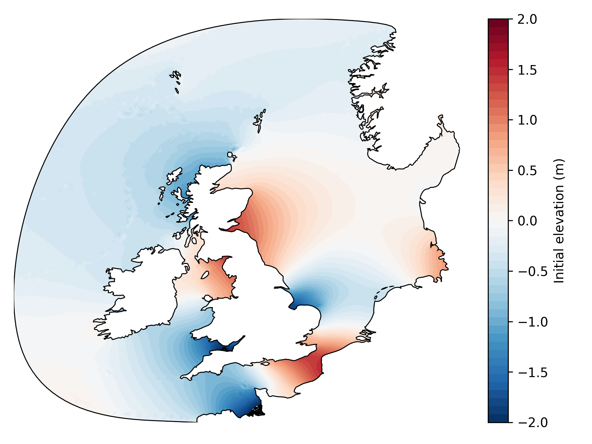
For the purposes of this demo, we have included HDF5 files containing spun-up elevation and velocity fields in the outputs_spinup directory. These can be used to initialise the model as follows. The spun-up HDF5 data were generated by a serial run, so this demo will not work in parallel.

solver_obj.load_state(14, outputdir="outputs_spinup", t=0, iteration=0)

The spin-up run was exported to HDF5 at daily intervals, so the first argument indicates that we resume on the fifteenth day (counting from zero). The last two keyword arguments are used to reset the clock for the subsequent simulation.

The final ingredient that we need is a callback function that updates the tidal forcings as the simulation progresses. With that, we are ready to run the model!

def update_forcings(t):
    tbnd.set_tidal_field(t)


solver_obj.iterate(update_forcings=update_forcings)

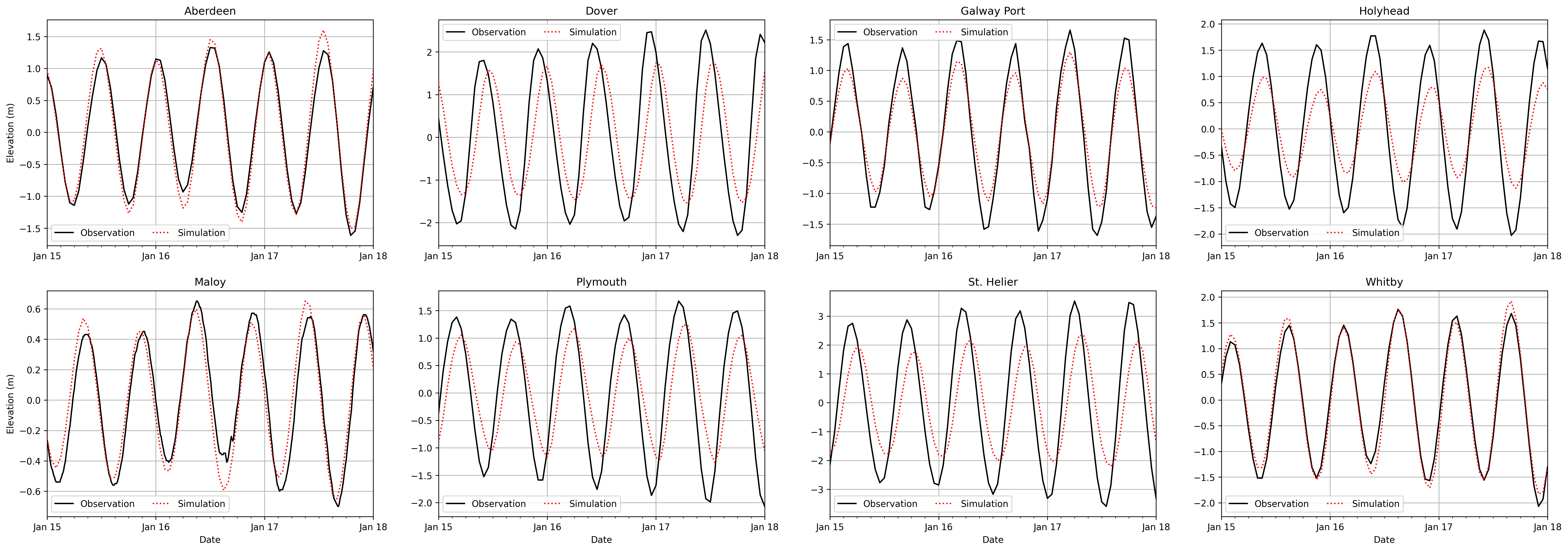
The elevation timeseries at the tide gauges should be as shown in the following plot, along with in-situ data from the CMEMS catalogue [Inf22]. Observe that the tidal cycles are well matched. The magnitudes are not so well matched. These results are generated on a coarse mesh, for the purposes of having a demo that can be run in a short amount of time. In order to more accurately approximate the observations, it would be beneficial to use a finer mesh. It could also be beneficial to calibrate the various parameters that define the tidal model, for example the Manning friction coefficient.

Scripts for generating all of the figures in this demo can be found in the example in the source code.

This tutorial can be dowloaded as a Python script here.

References

[AE09a]

Christopher Amante and Barry W Eakins. ETOPO1 arc-minute global relief model: procedures, data sources and analysis. NOAA National Centers for Environmental Information, 2009. Accessed 2022/03/14.

[AE09b]

Christopher Amante and Barry W Eakins. ETOPO1 arc-minute global relief model: procedures, data sources and analysis. noaa technical memorandum nesdis ngdc-24. National Geophysical Data Center, NOAA, 10(2009):V5C8276M, 2009. Accessed 2022/03/14.

[ACH+18]

Alexandros Avdis, Adam S Candy, Jon Hill, Stephan C Kramer, and Matthew D Piggott. Efficient unstructured mesh generation for marine renewable energy applications. Renewable Energy, 116:842–856, 2018.

[EE02]

Gary D Egbert and Svetlana Y Erofeeva. Efficient inverse modeling of barotropic ocean tides. Journal of Atmospheric and Oceanic technology, 19(2):183–204, 2002. Accessed 2022/03/14.

[Inf22]

E.U. Copernicus Marine Service Information. Atlantic-european north west shelf-ocean in-situ near real time observations. 2022. Accessed 2022/03/14. doi:10.48670/moi-00045.

[WS96]

Pål Wessel and Walter HF Smith. A global, self-consistent, hierarchical, high-resolution shoreline database. Journal of Geophysical Research: Solid Earth, 101(B4):8741–8743, 1996. Accessed 2022/03/14.